Authorship Attribution and Topic Discovery
Posted on Sat 02 December 2017 in nlp
As a project for Inference and Representation course in NYU, me and this guy decided to do some modeling of academic author interests. Such model would have several practical applications:
- Recommending latest papers to researchers, like what Mendeley and Microsoft Academic (MSA) does.
- Recommending the researchers to each other on some social network. Both Mendeley and MSA have this. I wonder why not a lot of people is using it as a social platform...
- Automatically assigning papers to reviewers. Actually we already have Toronto Paper Matching System (TPMS) adopted in multiple conference review systems.
Nonetheless, I have to admit that the main motivation (at least for me) of doing this project is to enable some ways to visualize the authors as groups, and inspect them with my own eyes. After all, it should be a lot of fun to see which researchers are close to each other on a figure.
The code is available here.
Dataset
Preferably, we would like a dataset that has strong indicator of "interest". A good example would be the user database of Mendeley or MSA, where actual users have an archive of papers; such papers obviously are of the user's interest. Another good dataset would be those from TPMS.
Unfortunately, it is unlikely for MSA and Mendeley to share their database to the public (of course). Also the dataset used by TPMS is not available. Therefore, we have to use authorship as a proxy of author interest. After all, a person should be sufficiently interested on some topic so that he/she can actually write something about it.
It is much easier to grab authorship data, since there are already a number of online libraries, such as arXiv and MSA. Both libraries have bulk data access Web API where one can easily scrape metadata of all the papers, including the authors, abstracts, titles, etc.
- We have a NIPS papers dataset, where Author Topic Model and the supervised version were both evaluated.
- Thanks to Andrej Karpathy's arxiv-sanity, we can conveniently grab thousands of machine learning research papers. We crawled 49,980 papers using arXiv-sanity, covering the research from 1997 to 2017 (a 20-year span).
For all datasets, we lowercase all the words, and removed the stop words.
Model
The model we were using is very simple:
- We represent each word and each author as 20-dimension embeddings, and compute a score of authorship by dot product between the author embedding and the average word embedding of a document.
- We minimize a pairwise ranking loss with negative sampling on both authors and documents.
More formally, we have a dataset of $D$ papers, where each document has a list of words $\mathcal{D}_i = (w_{i_1}, ..., w_{i_{n_i}})$ and a list of authors $\mathcal{A}_i = (a_{i_1}, ..., a_{i_{m_i}})$. The total number of authors in the dataset is $A$.
We first convert all $w_{i,j}$ and $a_{i,k}$ to some embedding vectors $\mathbf{w}_{i,j}$ and $\mathbf{a}_{i,k}$, using embedding matrices $\mathbf{W}$ and $\mathbf{A}$ for words and authors respectively. Then we compute the bag-of-words embedding and a bag-of-authors embedding:
The score is simply $s_i = \bar{\mathbf{w}}_i^T\bar{\mathbf{a}}_i$.
We chose ranking loss only because we don't feel like assigning a concrete number as a target for optimization. Rather, we think it makes more sense to just tell the model to "prefer" some authors/documents than others. In order to use ranking loss, we need some negative samples:
- For document, we simply sample one uniformly in the corpus and we can similarly have a bag-of-word $\bar{\mathbf{w}}_i'$.
- For authors, we treat the set of all authors, excluding $\mathcal{A}_i$, as the negative sample of authors. The formulation is simply
$$ \bar{\mathbf{a}}_i'=\dfrac{1}{A-m_i}\left(\sum_{k=1}^A\mathbf{a}_{i,k} - m_i \bar{\mathbf{a}}_i\right) $$
The loss function we are going to minimize is then simply two pairwise ranking losses, one for negative author samples and another for negative document samples, plus regularization terms:
where $\lambda_A = \lambda_W = 1\times 10^{-5}$.
We implemented the model in PyTorch. It's trainable on CPU, albeit very slowly. We believe that if we tailor the implementation in C or Fortran it will become a lot faster. Also, note that if we fix $\mathbf{W}$, the loss function would be convex w.r.t. $\mathbf{A}$, and vice versa. Not sure if doing alternating (stochastic) convex optimization would speed up.
Quantitative Results
-
We evaluated our model on the NIPS 1987-2013 dataset, same as what the Supervised Author-Topic Model did. We got our own set of papers from here. The resulting dataset is different from the original paper though: we have 2372 papers, 2577 authors and a vocabulary of 181948 words; the author set and the vocabulary is larger than theirs. Not sure if it helps the performance, but our model seems to be significantly better in terms of AUC on multiple authors:
Model AUC Supervised Author-Topic Model 0.67 Author-Topic Model 0.62 RF: Single-tree 0.55 RF: 5-trees 0.71 Ours 0.85 -
We also evaluated the average precision over 1, 5, 10, 50. The result is pretty lame though:
K AP@K 1 0.088 5 0.092 10 0.099 50 0.109 -
For each document-author pair in the dataset, we also computed the ranking of that author among everybody, and took the median. The result is 101 out of 2577 --- OK'ish, but not great.
Discovering Topics
We can do a lot of things as qualitative analysis: Given an author, propose a list of words associated to the topic of his/her interest. We can do that by ranking all the words $w_j$ with the scores $\mathbf{w}_j^T \mathbf{a}_i$. Given an author, find his/her nearest neighbors (or visualize the embeddings using t-SNE).
We evaluate qualitatively using the arXiv dataset. We first divided the dataset into training, validation, and test by 8:1:1. Then, we only keep the authors which appeared at least 3 times in the training set as the author set. We finally discard every paper in all three partitions where none of the authors is in the author set, and only kept the paper abstracts as documents. Consequently, we have:
- a vocabulary of 91719 words
- a set of 11492 authors
- a training set of 31923 papers
- a validation set of 3577 papers
- a test set of 3521 papers
Here is the top-ranked words given an author. Here I picked some authors that I have heard of, and grouped them into several categories. Yes, it means that I'm the noisy classifier of author interests.
I'm also considering releasing a web-app demo but I don't know if I have time to do it.
The meaning of $\lambda_c$ is explained in the following section.
| Name | Top-5 words | Top-5 words with $\lambda_c=0.1$ | Top-5 words with $\lambda_c=1$ |
|---|---|---|---|
| Li Fei-Fei | visual images image video object |
visual video object image images |
visual video object deep saliency |
| Kaiming He | image images networks neural deep |
deep image convolutional images visual |
video image visual 3d saliency |
| Seunghoon Hong | images proposed visual video object |
image images video segmentation visual |
video saliency 3d segmentation image |
| Rob Fergus | model models image images visual |
deep visual training neural object |
adversarial deep visual dropout video |
| Kyunghyun Cho | neural model language network word |
neural speech training deep word |
speech word rnn lstm sentiment |
| Chris Dyer | models language show word training |
language word text words translation |
word entity embedding translation sentiment |
| Tomas Mikolov | learning language word machine task |
language word text translation words |
word dialogue sentiment translation language |
| Samuel R. Bowman | model models neural language networks |
language word translation models text |
word translation dialogue speech language |
| Sergey Levine | learning approach training policy using |
policy learning reinforcement robot agents |
robot policy rl reinforcement reward |
| David Silver | learning algorithm policy algorithms problem |
policy agents reinforcement learning game |
policy agents rl reinforcement planning |
| Volodymyr Mnih | learning neural networks network deep |
neural deep networks reinforcement agents |
rl policy reinforcement robot agent |
| Pieter Abbeel | learning approach show policy training |
learning policy reinforcement agents robot |
policy rl robot reinforcement reward |
| David M. Blei | models model inference data bayesian |
inference bayesian models model latent |
causal bayesian inference latent variational |
| Daphne Koller | models inference bayesian model approach |
bayesian inference probabilistic uncertainty causal |
causal policy bayesian agents quantum |
| David Sontag | models data model inference algorithm |
inference models bayesian latent model |
latent ml variational inference predictive |
| Mehryar Mohri | algorithm problem algorithms learning show |
bounds algorithms algorithm optimization bound |
regret bounds fairness causal bound |
| Joan Bruna | networks network neural model deep |
networks network deep generative neural |
dropout kernel adversarial gans generative |
| Ian Goodfellow | learning neural training models deep |
learning neural deep adversarial training |
adversarial dropout gans generative gan |
| Nicolas Papernot | learning training data neural machine |
learning adversarial deep training machine |
adversarial dropout neurons gans genertive |
| Yann LeCun | training networks deep learning show |
deep training networks neural adversarial |
adversarial dropout deep gans gan |
| Yoshua Bengio | learning neural training networks models |
neural networks deep training learning |
adversarial dropout generative gans neurons |
| Geoffrey E. Hinton | data models learning model training |
models learning model neural training |
adversarial dropout generative gans rnn |
In the vanilla case (where there is no $\lambda_c$), it seems that other than the computer vision folks, the model tend to assign more generic words that can be applied to anybody (such as model, learning, etc.) as top-ranked words. This issue is more severe on the highest-ranked words: those words simply didn't tell us anything about the author's interest.
Inverse Document Frequency Regularizer?
Presumably, common words like model, learning should appear across a majority of the papers regardless of the actual topics. Since we have L2 regularization on the word embeddings, words that appear more often would have a larger L2 norm than the rare ones. And because we are computing the scores by dot products, the embeddings that have a bigger L2 norm will dominate the smaller ones. For instance, in the model above, the embedding for learning has an L2 norm of 23.06, while the one for policy is only 5.68.
Penalizing the norm of the more frequent words should help. However, we probably don't want to regularize a word that occurs frequently in a single document but nowhere else; such word is very likely informative. Therefore, we only want to penalize the word based on the number of documents where the word showed up. We can regard this idea as an analogy to inverse document frequency (IDF).
This regularization loss can be written as the following:
We evaluate the effect of this regularization both quantitatively and qualitatively. For comparison, we counted the number of different words occurred in top-$K$ ranking, and we compute the entropy of the normalized word occurrences. Those having a more diverse list of proposed words should have a higher entropy. We also give the median of author ranking and average precision to demonstrate how this regularization hurts our model:
| $\lambda_c$ | 0 | 0.1 | 1 |
|---|---|---|---|
| # of different words in top-1 | 76 | 101 | 84 |
| # of different words in top-5 | 159 | 221 | 207 |
| # of different words in top-10 | 234 | 332 | 314 |
| Entropy of top-1 word distribution | 2.95 | 3.34 | 3.45 |
| Entropy of top-5 word distribution | 4.04 | 4.38 | 4.34 |
| Entropy of top-10 word distribution | 4.55 | 4.88 | 4.81 |
| AP@1 | 0.027 | 0.023 | 0.017 |
| AP@5 | 0.020 | 0.018 | 0.012 |
| AP@10 | 0.023 | 0.021 | 0.014 |
| AP@50 | 0.028 | 0.026 | 0.017 |
| Median of ranking | 544 | 548 | 727 |
When I designed this IDF regularizer, I assumed that increasing $\lambda_c$ would consistently increase the "specificity" of word proposals. The experiment shows that buffing up $\lambda_c$ too much would instead kill off the diversity of proposals. In retrospect, this makes sense because the frequent-but-informative words get killed as well.
The top-ranked words for the authors with non-zero $\lambda_c$ is shown above. We can see that when $\lambda_c$ is too big, rare words did occur more frequently, even at the cost of killing the common-but-informative words:
adversarialandganseems to be all over the place.videois preferred overimage, even though the author did not publish a lot of works about video (e.g. Kaiming He).wordconsistently beatslanguage, although they sound equally informative to me (i.e. they are both significant indicator of NLP, but nothing more).- I don't know how
quantumgets in Daphne Koller's list.
Embedding visualizations
I tabulated the embeddings of authors which occurred more than 5 times:
Tensorflow Projector is an awesome tool as it runs T-SNE and PCA in your browser, and allows searching for nearest neighbor in terms of cosine distance or L2 distance. Feel free to search for your neighbors and evaluate my model's performance!
I also tabulated the words which occurred more than 5 times:
The PCA of the words looks like this:
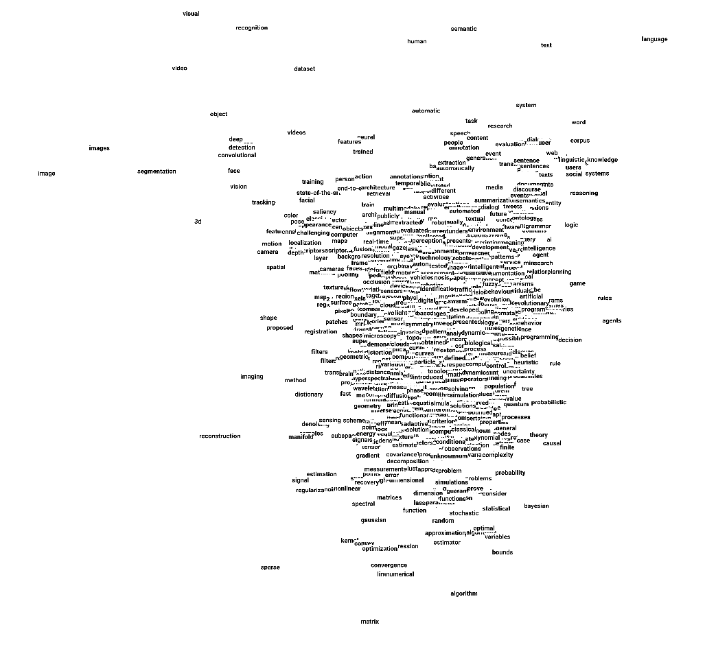
The result seems a bit satisfactory:
- Computer-vision-related words are placed on top left.
- Language-related words are placed at top right.
- The words at the top are more or less focused on practical applications.
- The words at the bottom seems all about theory and optimization.
- Interestingly, the word
state-of-the-artsits at the top-left, surrounded by computer vision words. This doesn't mean that getting state-of-the-art result in computer vision is easy, nor easier than other fields. - We can also see that the word
futuresits at the top-right, close to the NLP-ish words. This doesn't say that NLP is the only future.